Project
Hidden Outliers in Manifolds: Using Deep Learning to Generate Hard-to-Detect Anomalies
September 2023
The Problem with Outliers in High Dimensions
Douglas Hawkins defined an outlier as “an observation that deviates so much from other observations as to arouse suspicion that it was generated by a different mechanism.” Simple enough in two dimensions. You plot your data, spot the point that is far from everything else, and you are done.
But what happens when your data has 784 dimensions, like a 28x28 grayscale image? Or 3072 dimensions, like a small color image? The notion of “far from everything else” starts to break down. Distances become less meaningful. The curse of dimensionality makes traditional outlier detection unreliable.
And then there are hidden outliers: anomalies that look perfectly normal when you examine the full feature space, but reveal their true nature only when you look at specific subsets of features. These are the outliers that slip through conventional detection methods. They are also, it turns out, exactly the kind of anomalies you encounter in real problems like fraud detection, infrastructure monitoring, and healthcare analytics.
This post describes my bachelor thesis work on generating hidden outliers using deep learning and manifold learning. The core insight is that by projecting high-dimensional data onto a learned manifold, we can efficiently generate hidden outliers that would be computationally infeasible to produce in the original space.
What Makes an Outlier “Hidden”?
To understand hidden outliers, you need to think about outlier detection from multiple perspectives, what researchers call the “multiple views” property.
Consider a financial transaction dataset with features like amount, time, location, and merchant category. A transaction might look completely normal when you examine each feature individually. The amount is within normal range. The time is during business hours. The location is in a city where the customer has shopped before. But when you look at the specific combination of a high amount, at midnight, from a location the customer has never visited, the transaction suddenly looks suspicious.
This is the essence of hidden outliers. They are outliers in some subspaces but inliers in others.
More formally, imagine you have an outlier detection model trained on your full dataset. Call this the “full-space model.” Now imagine training separate outlier detection models on every possible subset of features, what we call the “subspace ensemble.” A hidden outlier is a point where these two perspectives disagree: either the full-space model says “normal” while some subspace model says “outlier,” or vice versa.
The region where these models disagree is called the “hidden region” or “area of disagreement.” Points in this region are hidden outliers.
The Computational Challenge
Here is the problem: if your dataset has d features, the number of possible subspaces is 2^d. For a 784-dimensional MNIST image, that is more subspaces than atoms in the observable universe. You cannot fit an outlier detection model on every subspace. It is computationally impossible.
Previous work on hidden outlier generation, like the HIDDEN algorithm, addressed this by randomly sampling subspaces and using heuristics to place outliers. But these approaches struggle with high-dimensional data and often require sensitive hyperparameter tuning.
The BISECT algorithm, which forms the backbone of my thesis, improved on this by using a bisection method to efficiently find points in the hidden region. But even BISECT hits a wall when dimensionality gets high enough.
My thesis asks: what if we did not work in the original high-dimensional space at all? What if we projected the data onto a lower-dimensional manifold first?
Manifolds and Autoencoders
A manifold is a mathematical space that locally resembles Euclidean space. The classic example is the surface of the Earth: globally it is a sphere, but locally (at human scales) it looks flat. High-dimensional data often lies on or near a lower-dimensional manifold embedded in the full space. Images of handwritten digits, for instance, do not fill the entire 784-dimensional space. They cluster on a much lower-dimensional structure determined by the strokes and shapes that make up valid digits.
Autoencoders are neural networks designed to learn these manifolds. An autoencoder has two parts: an encoder that compresses input data into a low-dimensional “latent space,” and a decoder that reconstructs the original data from this compressed representation. If the reconstruction is good, the latent space has captured the essential structure of the data.
| Autoencoder Type | Architecture | Best For |
|---|---|---|
| Normal (NAE) | Dense layers only | Tabular data |
| Variational (VAE) | Dense + sampling | Generation tasks |
| Convolutional (CAE) | Conv layers | Image data |
| Deep Convolutional (DCAE) | Conv + dense bottleneck | Controlled latent dims |
The key insight is that if we generate hidden outliers in the latent space, we are working with a tractable number of dimensions (say, 8 or 16) instead of hundreds or thousands. We can then decode these latent outliers back to the original space.
The Approach
My approach combines autoencoders with the BISECT algorithm:
- Train an autoencoder on the dataset to learn a low-dimensional manifold representation.
- Encode the data into the latent space.
- Run BISECT on the encoded data to generate hidden outliers in the latent space.
- Decode the generated outliers back to the original space.
For outlier detection, the generated hidden outliers can serve as a synthetic “positive class” for training a classifier. This turns unsupervised anomaly detection into a supervised problem, which often improves performance.
The BISECT Algorithm
BISECT works by finding points in the “area of disagreement” between the full-space and subspace outlier models. Here is how it operates:
Origin Selection: Start from a point that is an inlier in the full-space model. The “weighted” method selects origins with probability proportional to their outlierness score, focusing the search near the boundary between inliers and outliers.
Direction: Pick a random direction by sampling from a d-dimensional unit sphere.
Bisection: Starting from the origin, move along the direction and use binary search to find the boundary where the outlier status changes. Points at this boundary are hidden outliers.
The algorithm is elegant because it does not require exhaustive search through all subspaces. It exploits the geometric structure of the hidden region to find outliers efficiently.
I implemented BISECT in Python and released it as an open-source library. The implementation is compatible with any outlier detection method from the PyOD library and handles the memory challenges of fitting models on many subspaces by storing fitted models on disk.
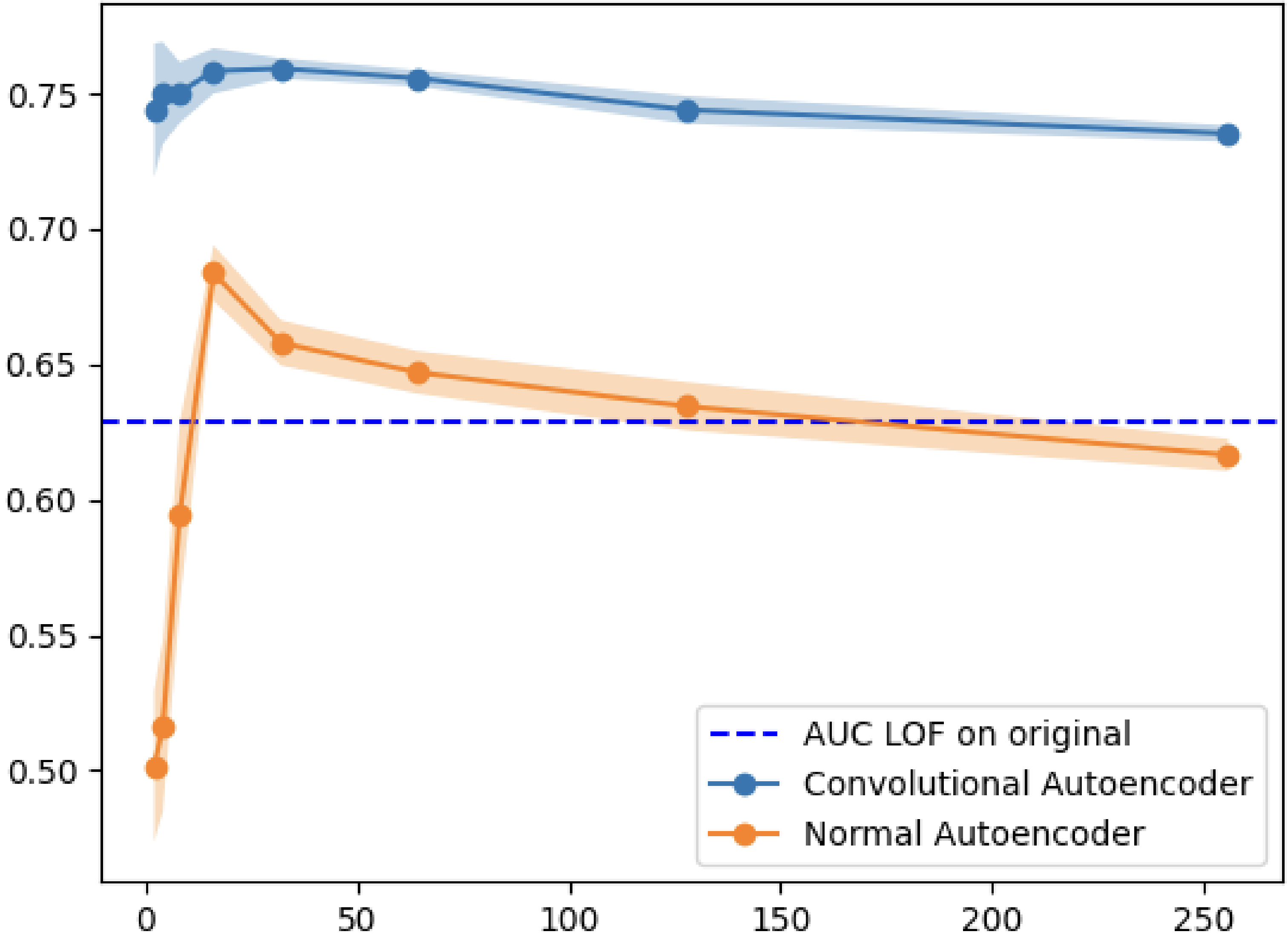
Experiment 1: LOF on Manifolds vs. Full Space
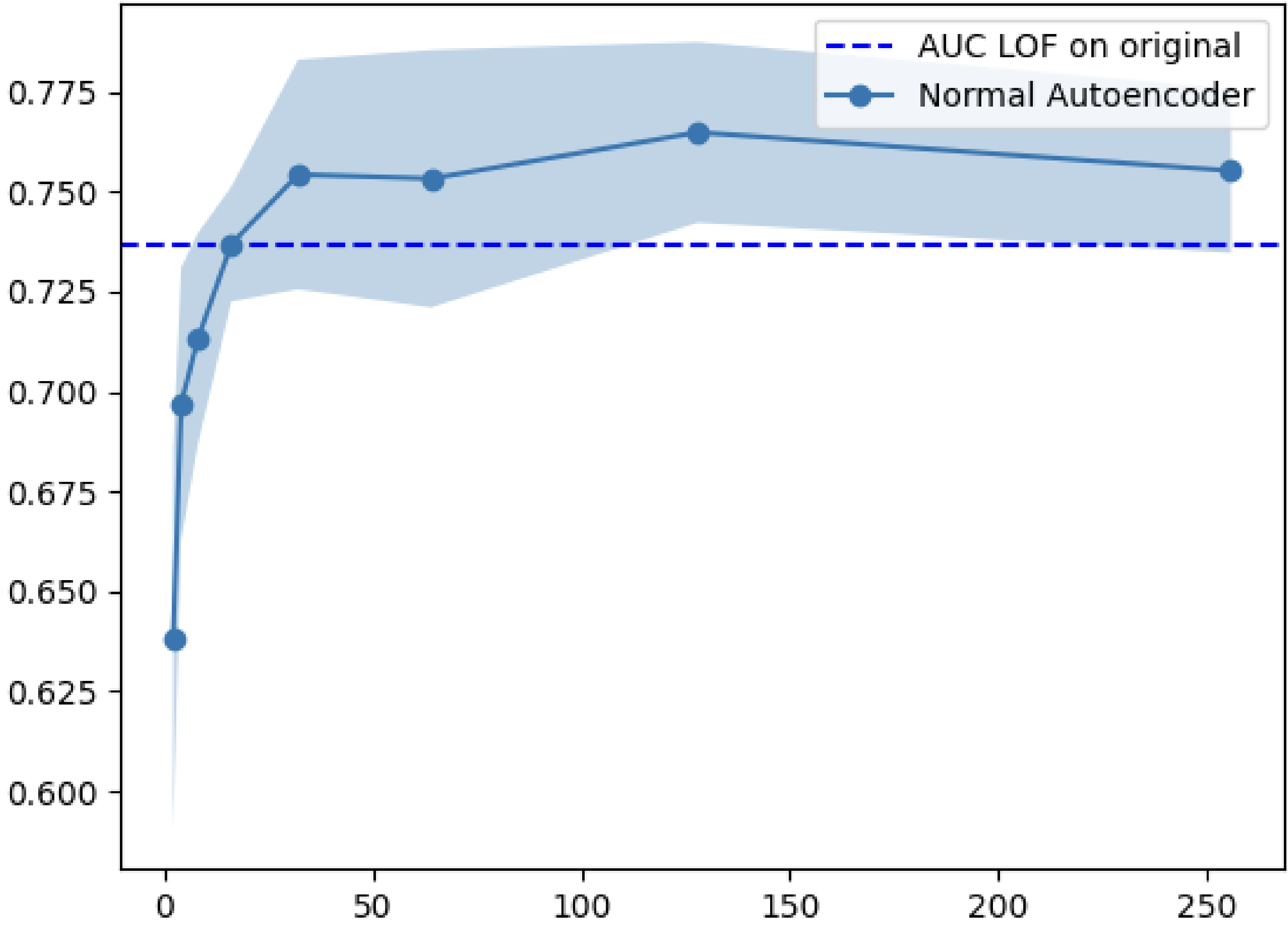
My first experiment tested whether outlier detection improves when applied to the latent space rather than the original space. I trained various autoencoders on five datasets (MNIST, Fashion-MNIST, CIFAR10, Arrhythmia, Internet Ads) and compared Local Outlier Factor (LOF) performance on the encoded vs. original data.
| Dataset | Best Autoencoder | Latent Dims | LOF on Latent | LOF on Full | Improvement |
|---|---|---|---|---|---|
| MNIST | CAE | 32 | 0.760 | 0.629 | +20.8% |
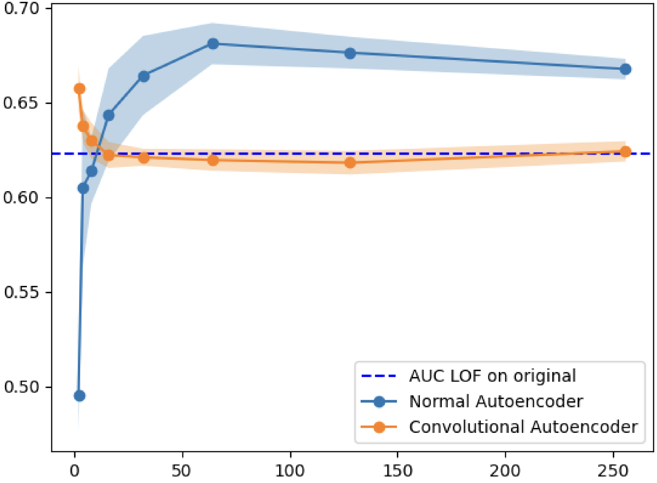
| Fashion-MNIST | NAE | 64 | 0.682 | 0.623 | +9.5% |
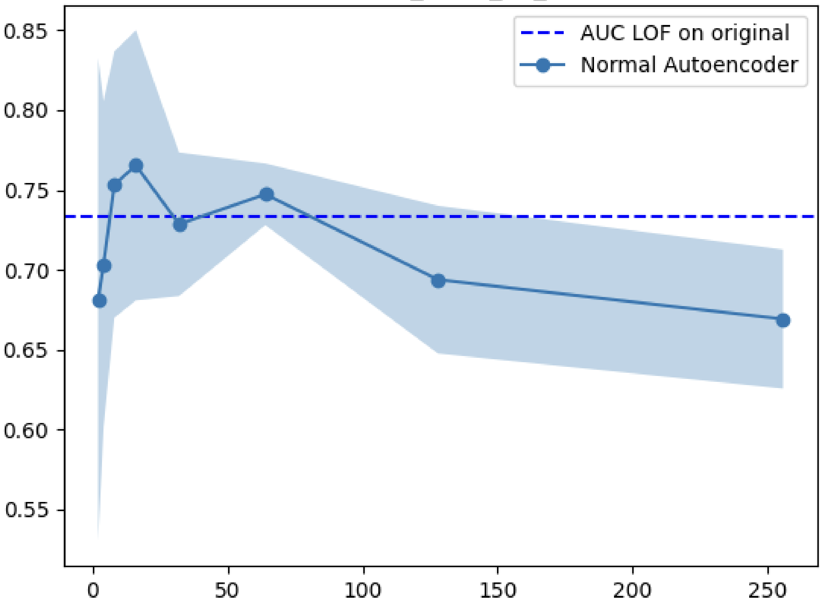
| Arrhythmia | NAE | 16 | 0.762 | 0.734 | +3.8% |
| Internet Ads | NAE | 128 | 0.766 | 0.737 | +3.9% |
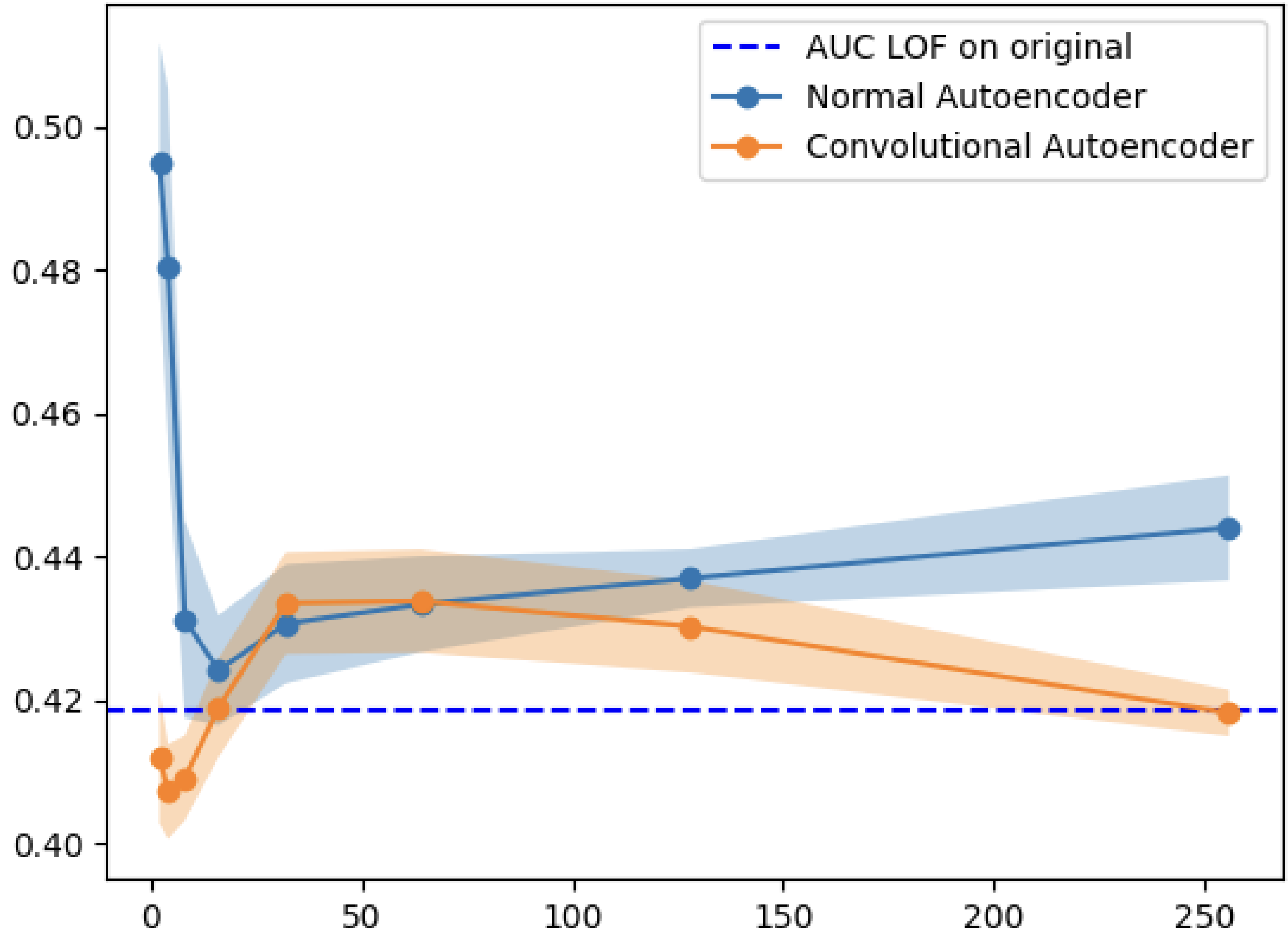
| CIFAR10 | VAE | 128 | 0.504 | 0.419 | +20.3% |
The results were clear: LOF on the latent space consistently outperformed LOF on the full space. The improvement was especially pronounced for image datasets, where the original dimensionality is highest.
I also compared against more sophisticated methods like DeepSVDD, AnoGAN, and MO-GAAL. Surprisingly, simple LOF on autoencoder latent spaces often matched or exceeded these complex approaches.
Why does this work? Autoencoders learn to map data onto a manifold that preserves meaningful structure while discarding noise. Outliers, which deviate from the normal data distribution, get mapped to sparse regions of the latent space. Since LOF measures local density deviation, it becomes more effective when the data lives in a space where density differences are more pronounced.
Why do variational autoencoders underperform? VAEs add stochastic noise during encoding and include a KL divergence term in their loss function that pushes the latent distribution toward a standard normal. This can blur the distinction between inliers and outliers, hurting detection performance.
Experiment 2: Hidden Outliers for Anomaly Detection
Can we use BISECT-generated hidden outliers to improve anomaly detection? The idea is to train a classifier (Random Forest) with the encoded normal data as the negative class and the generated hidden outliers as the positive class. Then use this classifier to detect real outliers.
The methodology:
- Encode the dataset (containing some outliers) with an autoencoder.
- Generate hidden outliers using BISECT on the encoded data.
- Train a Random Forest: encoded real data = class 0, generated hidden outliers = class 1.
- Evaluate on the real outliers in the dataset.
| Dataset | Autoencoder | Latent Dims | RF + BISECT | LOF Encoded | LOF Full |
|---|---|---|---|---|---|
| MNIST 7 vs 1 | DCAE | 16 | 0.957 | 0.626 | 0.586 |
| MNIST 9 vs 0 | DCAE | 8 | 0.902 | 0.636 | 0.483 |
| Fashion outlier 2 | DCAE | 8 | 0.749 | 0.589 | 0.623 |
| Arrhythmia | NAE | 2 | 0.689 | 0.639 | 0.734 |
The results were mixed but illuminating. For image datasets (MNIST, Fashion-MNIST), the approach worked remarkably well, with AUC scores above 0.9 in some configurations. For tabular datasets like Arrhythmia and Internet Ads, simple LOF on the full space often performed better.
This suggests the approach is particularly valuable when the data has high intrinsic dimensionality and complex structure that autoencoders can capture, exactly the settings where traditional methods struggle most.
I also tested whether the ratio of generated outliers to real data matters. Surprisingly, it did not. Whether I generated 1x, 1.5x, 2x, or 3x the number of data points as hidden outliers, performance remained similar. This makes sense: BISECT generates outliers near real data points, so generating more outliers likely adds redundant information rather than new signal.
Experiment 3: Novelty Detection
Novelty detection is a slightly different problem: train on data containing only “normal” examples, then detect anomalies in new data. This is the realistic scenario for many applications where you know what normal looks like but cannot enumerate all possible anomalies.
I modified the setup:
- Split data into training (inliers only) and test (inliers + outliers).
- Train autoencoder on training data.
- Generate hidden outliers using BISECT on encoded training data.
- Train Random Forest on training data as negative, hidden outliers as positive.
- Evaluate on encoded test data.
| Dataset | Autoencoder | Latent Dims | RF + BISECT | LOF Full |
|---|---|---|---|---|
| CIFAR10 class 5 vs 0 | DCAE | 8 | 0.684 | 0.639 |
| Fashion class 5 vs 0 | VAE | 4 | 0.679 | 0.440 |
| MNIST class 5 vs 0 | DCAE | 4 | 0.780 | 0.462 |
| Arrhythmia | NAE | 32 | 0.695 | 0.125 |
The novelty detection results were encouraging. In most cases, the BISECT approach outperformed LOF on the full space, sometimes dramatically. The Arrhythmia result is particularly striking: the approach achieved 0.695 AUC where LOF on full space managed only 0.125.
What Do Hidden Outliers Look Like?
One question that motivated this work: if we generate hidden outliers in image data, what do they actually look like?
I ran an exploratory experiment where I:
- Trained autoencoders on MNIST with 12 latent dimensions.
- Generated 10,000 hidden outliers in the latent space.
- Decoded them back to images.
- Also generated hidden outliers directly in the 784-dimensional pixel space.
- Compared the results.
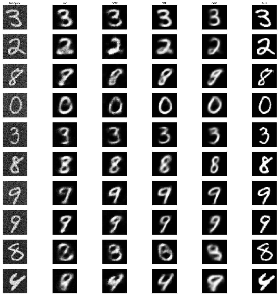
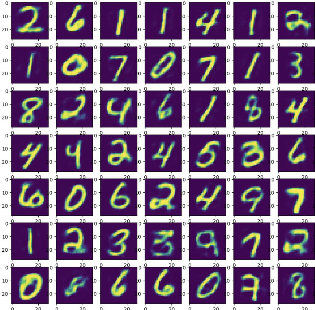
The results were visually striking. Hidden outliers generated in the latent space and decoded look like slightly distorted but recognizable digits. The decoder acts as a kind of “denoiser,” mapping the outliers back onto the manifold of plausible images.
Hidden outliers generated directly in the high-dimensional pixel space look like random noise added to the original image. Because BISECT in my implementation only considers 2^12 subspaces (a tiny fraction of the 2^784 possible), it cannot detect that the noisy pixels might be outliers in other subspaces. The result is that the “outlierness” is spread across many unexamined subspaces as random noise.
This highlights why working in the latent space matters. The manifold learned by the autoencoder concentrates the meaningful variation into a small number of dimensions, making hidden outlier generation tractable and meaningful.
The Python Library
As part of this thesis, I developed and released a Python implementation of BISECT:
GitHub: github.com/dschulmeist/hidden-outlier-generation
PyPI: Available as hidden-outlier-generation
The library supports:
- Multiple origin selection methods (random, weighted, centroid, least outlier)
- Any outlier detector from PyOD
- Efficient disk-based storage for fitted subspace models
- Configurable subspace limits for high-dimensional data
One of the main implementation challenges was memory management. Fitting outlier detection models on thousands of subspaces creates massive memory pressure, especially with parallel processing. The solution was to store fitted models on disk and load them as needed, trading some speed for the ability to handle large datasets.
Limitations and Future Directions
This work has clear limitations that point toward future research:
Hyperparameter sensitivity: I did not extensively tune autoencoder architectures or training hyperparameters. Different datasets might benefit from different configurations. A systematic architecture search could improve results.
Limited datasets: The experiments covered five datasets. Broader evaluation across more domains would strengthen the conclusions.
Autoencoder choice: The finding that variational autoencoders underperform deserves deeper investigation. Perhaps different VAE formulations or training procedures could address this.
Subspace limits: BISECT’s subspace limit (2^12 in my experiments) is a hard constraint. For very high-dimensional data, even this might be insufficient. Smarter subspace selection strategies could help.
Decoder effects: The decoder appears to “denoise” hidden outliers, pulling them back toward the data manifold. Understanding and controlling this effect could lead to better outlier generation.
Conclusion
This thesis explored the intersection of manifold learning, deep learning, and hidden outlier generation. The key findings:
-
Outlier detection improves on learned manifolds. Applying LOF to autoencoder latent spaces consistently outperformed applying it to the original high-dimensional space.
-
BISECT works well on manifolds. Generating hidden outliers in the latent space is computationally tractable and produces meaningful anomalies when decoded.
-
Hidden outliers can improve detection. Using generated hidden outliers as a positive class for supervised learning showed promising results, especially for image data.
-
The approach is accessible. The released Python library makes it easy to experiment with hidden outlier generation on new datasets.
The broader implication is that manifold learning can make previously intractable problems tractable. By projecting data onto a learned low-dimensional space, we can apply algorithms that would be computationally impossible in the original space. This principle extends beyond outlier detection to many areas of high-dimensional data analysis.
This post is based on my bachelor thesis completed at Karlsruhe Institute of Technology in September 2023